Dijkstra's Algorithm

Computational Mathematics

02

Important Notice

This is an unofficial support material, created by students with the help of artificial intelligence. It does not represent the official position of the institution or its professors.
Do not question or bother the professors about this content. The material is based on notes taken during classes and supplementary research done by the students themselves.
This material may contain inaccuracies. When in doubt, always refer to the official material provided by the professor and the references listed at the end.
Suggestions and Corrections
Found an error or have a suggestion? Send your contribution through the class WhatsApp group. All collaboration is welcome to improve the material for everyone.
03
TABLE OF CONTENTS

Contents

04
INTRO

Finding the Shortest Path

Imagine you need to travel from Dublin to Cork. There are many possible routes — some faster, some shorter, some cheaper on fuel. This is a path finding problem: given a network of locations connected by roads, find the "best" route from one point to another. "Best" could mean least time, least distance, most bandwidth, or least cost — these are all optimisation problems.

We can model these networks as weighted graphs: locations become nodes (also called vertices), roads become edges, and each edge has a weight — a number representing its cost (distance, time, etc.). An algorithm is simply a step-by-step series of instructions to solve a problem. Dijkstra's Algorithm (pronounced "Dike-stra", after Dutch computer scientist Edsger Dijkstra) is one of the most famous algorithms for finding the shortest path in a weighted graph.

The objective is simple: find one sequence of nodes connecting a start node to an end node that has the least combined edge weight. Dijkstra's approach works by exploring outward from the start node, always picking the closest unvisited neighbour first, and gradually building up a table of shortest known distances. By the time it reaches the destination, it guarantees the path is optimal.

05
DIAGRAM

Why Do We Need an Algorithm?

The brute-force approach does not scale

Brute Force

Try every possible path from A to H, calculate each total cost, pick the shortest.

7 nodesHundreds of paths
100 nodesMillions of paths
1,000 nodesMore paths than atoms in the universe
Dijkstra's Algorithm

Visit nodes smartly — always pick the closest unvisited node next. Each node is visited at most once.

7 nodes7 steps
100 nodes~100 steps
1,000 nodes~1,000 steps
06
DIAGRAM

Weighted Graph

The graph we'll use to trace Dijkstra's algorithm

21133652ABCDEFH

Each number on an edge represents the cost of travelling between two nodes

07
DIAGRAM

The Algorithm

Four steps to find the shortest path

1Start at the source node. Set its distance to 0. All other distances =
2Look at all unvisited neighbours. Calculate: current distance + edge weight
3If the new distance is shorter, update the distance table
4Mark current node as visited. Move to the unvisited node with the smallest distance. Repeat from step 2
08
DIAGRAM

Step 0 — Start at Node A

Initialise distances and begin

We begin at node A with distance 0. All other nodes start at ∞ (infinity). From A, we can reach B (cost 2) and C (cost 1). We add both to our queue.
2 1 1 3 3 6 5 2 A0 B2 C1 D E F H
09
DIAGRAM

Step 1 — Visit Node C (cost 1)

C has the smallest distance in the queue

Node C has the smallest distance (1), so we visit it next. From C, we can reach D (1+3=4) and F (1+6=7). B is already queued with distance 2, which is still valid.
2 1 1 3 3 6 5 2 A0 B2 C1 D4 E F7 H
10
DIAGRAM

Step 2 — Visit Node B (cost 2)

B has the smallest distance among unvisited nodes

Node B (distance 2) is next. From B, we reach D (2+1=3) — this is shorter than D's current distance of 4! We update D to 3. We also reach E (2+3=5).
2 1 1 3 3 6 5 2 A0 B2 C1 D4→3 E5 F7 H
11
DIAGRAM

Step 3 — Visit Node D (cost 3)

D's neighbours are already visited — no updates

Node D (distance 3) is next. Both of D's neighbours (B and C) are already visited. No distance updates — we simply mark D as visited and move on.
2 1 1 3 3 6 5 2 A0 B2 C1 D3 E5 F7 H
12
DIAGRAM

Steps 4 & 5 — Visit E (cost 5), then F (cost 7)

Getting closer to H

Node E (distance 5) is visited next. From E we check F: 5+5=10, but F already has distance 7, so no update. Then we visit F (distance 7). From F we reach H (7+2=9)!
2 1 1 3 3 6 5 2 A0 B2 C1 D3 E5 F7 H9
13
DIAGRAM

Result — Shortest Path Found!

A → C → F → H with total cost 9

The algorithm is complete! The shortest path from A to H is A → C → F → H with total cost 9 (1 + 6 + 2). Notice this goes through C and F, not through B — even though B is closer to A, the path through B leads to a longer total route.
2 1 1 3 3 6 5 2 A0 C1 F7 H9 B2 D3 E5
14
DIAGRAM

Worked Example 2 — A Larger Graph

Finding the shortest path from S to T in a 7-node graph

New graph, same algorithm. This graph has 7 nodes and 11 edges — more complex than our first example. The edges from S reach three neighbours: A (cost 7), B (cost 2), and C (cost 3). Watch the algorithm explore outward from S.
72334411835S0ABCDET
15
DIAGRAM

Worked Example 2 — Animated Walkthrough

Watch Dijkstra find the path from S to T

Watch the animation: The algorithm explores outward from S, visiting nodes in order of their distance. Notice how it discovers the path S → B → E → T (cost 6) — even though A and D are explored, they don't lead to a shorter path to T.
7 2 3 3 4 4 1 1 8 3 5 S A B C D E T 0 7 5 2 3 6 3 6 Shortest path: S → B → E → T (cost 6)
16
DIAGRAM

Worked Example 2 — Column Walkthrough

Step-by-step columns for S to T

Start at S
(cost 0)
SA: 0+7 = 7 NEW
SB: 0+2 = 2 NEW
SC: 0+3 = 3 NEW
→ Select B (2) 2
Visit B
(cost 2)
BD: 2+4 = 6 NEW
BE: 2+1 = 3 NEW
A: 7 2+3 = 5
→ Select C (3) 3
Visit C
(cost 3)
CB: 3+1 = 4 > 2 (no update)
CE: 3+8 = 11 > 3 (no update)
→ Select E (3) 3
Visit E
(cost 3)
ET: 3+3 = 6 NEW
→ Select A (5) 5
Visit A
(cost 5)
AD: 5+4 = 9 > 6 (no update)
→ Select D (6) 6
Visit D
(cost 6)
DT: 6+5 = 11 > 6 (no update)
→ Select T (6) 6
Shortest path: S → B → E → T, total cost = 6 (2 + 1 + 3)
17
DIAGRAM

Worked Example 3 — Finding All Shortest Paths

Sometimes the journey matters more than the destination

New goal: This time we find the shortest path from P to every node — not just one target. This is useful when you need to reach multiple destinations, like a delivery van planning its route.
14263512P0QRSTU
18
DIAGRAM

Worked Example 3 — Full Dijkstra Run

Finding shortest paths from P to all nodes

All shortest paths found! Notice that every shortest path goes through Q and R — they're the 'gateway' nodes. This pattern is common in real networks: some nodes are more important than others for efficient routing.
1 4 2 6 3 5 1 2 P Q R S T U 0 1 4 3 7 6 8 7
DestinationShortest DistancePath
Q1P → Q
R3P → Q → R
S6P → Q → R → S
T8P → Q → R → T
U7P → Q → R → S → U
19
DIAGRAM

Worked Example 3 — Column Walkthrough

Step-by-step columns for P to all nodes

Start at P
(cost 0)
PQ: 0+1 = 1 NEW
PR: 0+4 = 4 NEW
→ Select Q (1) 1
Visit Q
(cost 1)
R: 4 1+2 = 3
QS: 1+6 = 7 NEW
→ Select R (3) 3
Visit R
(cost 3)
S: 7 3+3 = 6
RT: 3+5 = 8 NEW
→ Select S (6) 6
Visit S
(cost 6)
SU: 6+1 = 7 NEW
→ Select U (7) 7
Visit U
(cost 7)
(no unvisited neighbours)
→ Select T (8) 8
All shortest paths found from P: Q=1, R=3, S=6, U=7, T=8
20
DIAGRAM

Step-by-Step Walkthrough

Running Dijkstra from A to H — following the algorithm

Start at A
(cost 0)
AB: 0+2 = 2 NEW
AC: 0+1 = 1 NEW
→ Select C (1) 1
Visit C
(cost 1)
AB: 2 (unchanged)
CD: 1+3 = 4 NEW
CF: 1+6 = 7 NEW
→ Select B (2) 2
Visit B
(cost 2)
4 2+1 = 3
BE: 2+3 = 5 NEW
CF: 7 (unchanged)
→ Select D (3) 3
Visit D
(cost 3)
BE: 5 (unchanged)
CF: 7 (unchanged)
(no new paths)
→ Select E (5) 5
Visit E
(cost 5)
CF: 7 (unchanged, 5+5=10 > 7)
→ Select F (7) 7
Visit F
(cost 7)
FH: 7+2 = 9 NEW
→ Select H (9) 9
Shortest path: A → C → F → H, total cost = 9 (1 + 6 + 2)
21
DIAGRAM

Dijkstra vs A* — Grid Comparison

Same map, same cost — but look at how many nodes each algorithm visits
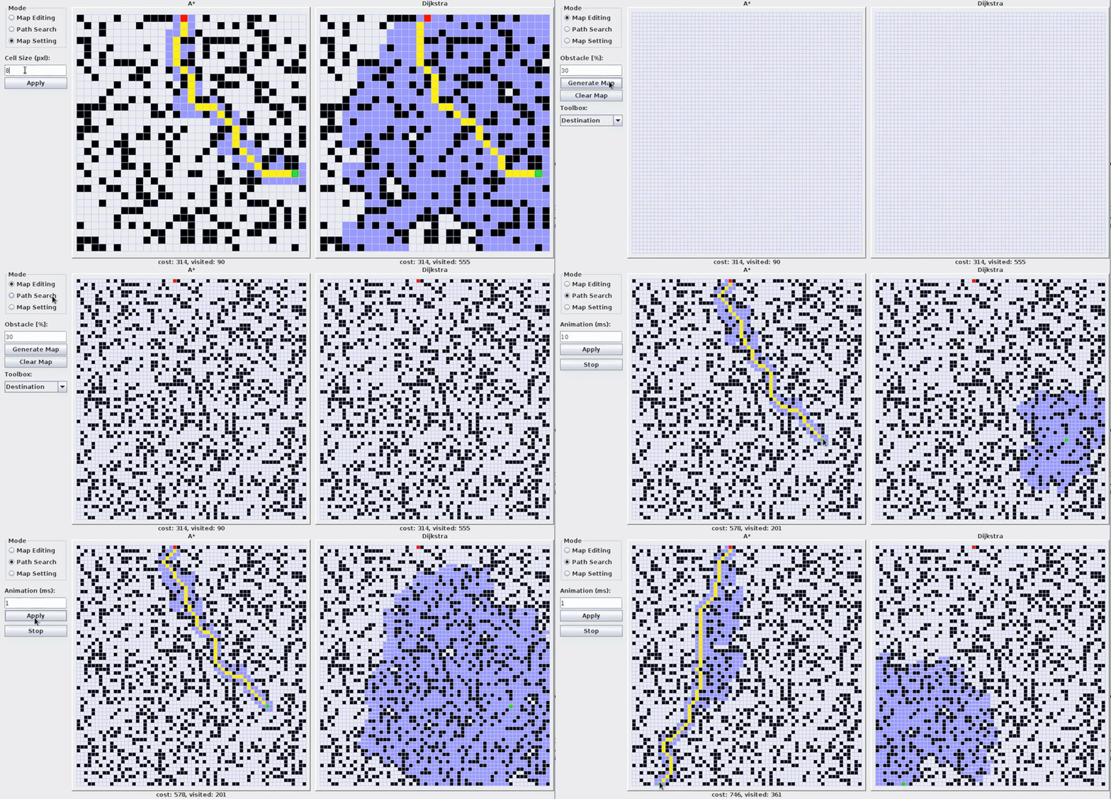
What to watch for: Both algorithms find a path with the same cost. The purple/blue shading shows which nodes each algorithm explored. Notice how Dijkstra (right) floods the entire grid, while A* (left) heads straight for the goal — it uses a heuristic (estimated distance to target) to guide its search.
Side-by-side comparison of Dijkstra and A* on a grid map

A* visited 90 nodes. Dijkstra visited 555 — over 6 times more. Video by Kevin Wang.

A* visited 90 nodes. Dijkstra visited 555 — over 6 times more. Video by Kevin Wang.

22
DIAGRAM

Dijkstra vs A* — Real-World Comparison

Watch Dijkstra explore every street in Rome before finding the path
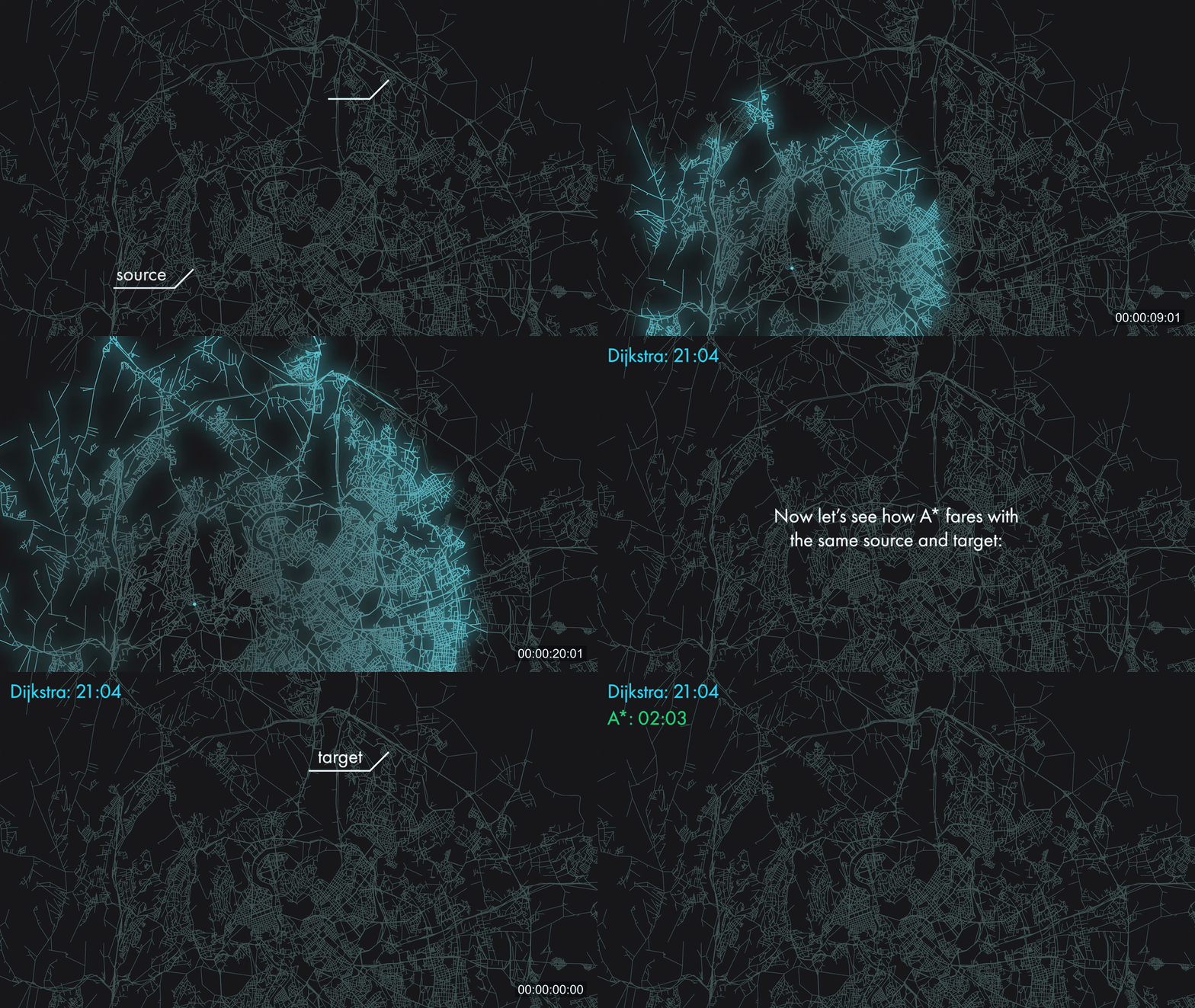
Real-world impact: This is Dijkstra running on actual road data from Rome, Italy (OpenStreetMap). Watch the cyan glow expand in every direction from the source — Dijkstra explores every street, alley, and dead end equally. It took 21 minutes to find the path. A* found the exact same path in just 2 minutes by prioritising roads that lead towards the target. This is why modern GPS systems use A* or similar heuristic algorithms, not pure Dijkstra.
Dijkstra vs A* pathfinding comparison on the streets of Rome

Dijkstra took 21:04 to find the path. A* found the same path in just 02:03. Video by Anthony Madorsky.

Dijkstra took 21:04 to find the path. A* found the same path in just 02:03. Video by Anthony Madorsky.

23
DIAGRAM

Dijkstra vs A* — Understanding the Difference

Two algorithms, one goal — but very different strategies

Dijkstra’s Algorithm
  • Explores nodes in ALL directions equally
  • Guaranteed to find the shortest path
  • No knowledge of where the target is
  • Like a ripple spreading in a pond
  • Visits many unnecessary nodes
A* Algorithm
  • Explores towards the target first
  • Also guaranteed shortest path (with admissible heuristic)
  • Uses a heuristic — estimated distance to target
  • Like following a compass towards your destination
  • Visits far fewer nodes
The Key Difference: The Heuristic

A* adds one extra piece of information: an estimate of how far each node is from the target. Instead of picking the node with the smallest distance from start (like Dijkstra), A* picks the node with the smallest distance from start + estimated distance to target. This simple addition dramatically reduces the number of nodes explored.

FeatureDijkstraA*
Uses heuristic?NoYes
Finds shortest path?AlwaysYes (with admissible heuristic)
SpeedSlower (explores everything)Faster (focused search)
Memory usageHigherLower
Best forAll shortest paths from one sourceSingle source to single target
Used inNetwork routing, database queriesGPS navigation, video games
24
DIAGRAM

Real-World Applications

Where shortest path algorithms power our daily lives

GPS Navigation

Every time you ask Google Maps or Apple Maps for directions, a variant of Dijkstra’s algorithm runs on millions of road segments. The edges are roads, weights are travel times (updated in real-time with traffic data), and the algorithm finds the fastest route. Modern GPS uses A* with geographical distance as the heuristic.

Internet Routing

When you send a message on WhatsApp, it travels through multiple routers to reach its destination. Protocols like OSPF (Open Shortest Path First) use Dijkstra’s algorithm to find the fastest path through the network. Each router is a node, each connection is an edge weighted by latency or bandwidth.

Video Games

In games like Age of Empires, Civilization, or any strategy game, units need to navigate around obstacles to reach their destination. A* is the standard pathfinding algorithm in game development. It runs thousands of times per second to move characters, enemies, and NPCs around the map.

Social Networks

LinkedIn’s ‘degrees of connection’ and Facebook’s ‘People You May Know’ use graph algorithms to find short paths between users. The ‘six degrees of separation’ concept is essentially a shortest path problem on a social graph with billions of nodes.

25
CODE

Dijkstra's Algorithm in Java

Using a priority queue to find the shortest path

DijkstraAlgorithm.java
import java.util.*;

public class DijkstraAlgorithm {
    
    // Find shortest distances from start to all nodes
    public static int[] dijkstra(int[][] graph, int start) {
        int n = graph.length;
        int[] distances = new int[n];
        boolean[] visited = new boolean[n];
        
        // Initialise all distances to "infinity"
        Arrays.fill(distances, Integer.MAX_VALUE);
        distances[start] = 0;
        
        // Priority queue: {distance, node}
        PriorityQueue<int[]> queue = 
            new PriorityQueue<>(Comparator.comparingInt(a -> a[0]));
        queue.offer(new int[]{0, start});
        
        while (!queue.isEmpty()) {
            int[] current = queue.poll();
            int dist = current[0], node = current[1];
            
            if (visited[node]) continue;
            visited[node] = true;
            
            // Check all neighbours
            for (int next = 0; next < n; next++) {
                if (graph[node][next] > 0 && !visited[next]) {
                    int newDist = dist + graph[node][next];
                    if (newDist < distances[next]) {
                        distances[next] = newDist;
                        queue.offer(new int[]{newDist, next});
                    }
                }
            }
        }
        return distances;
    }
}
Main.java
public class Main {
    public static void main(String[] args) {
        // Adjacency matrix — 0 means no direct connection
        //          A  B  C  D  E  F  H
        int[][] graph = {
            {0, 2, 1, 0, 0, 0, 0},  // A
            {2, 0, 0, 1, 3, 0, 0},  // B
            {1, 0, 0, 3, 0, 6, 0},  // C
            {0, 1, 3, 0, 0, 0, 0},  // D
            {0, 3, 0, 0, 0, 5, 0},  // E
            {0, 0, 6, 0, 5, 0, 2},  // F
            {0, 0, 0, 0, 0, 2, 0}   // H
        };
        String[] nodes = {"A","B","C","D","E","F","H"};
        
        int[] distances = DijkstraAlgorithm.dijkstra(graph, 0);
        
        // Print shortest distances from A
        for (int i = 0; i < nodes.length; i++) {
            System.out.println("A → " + nodes[i] + " = " + distances[i]);
        }
        // Output: A → H = 9
    }
}
26
SUMMARY

Quick Reference

ConceptNotationMeaning
Node (Vertex)A, B, C...A point/location in the graph
EdgeA—BA connection between two nodes
Weightw(A,B) = 3The cost of travelling along an edge
Weighted GraphG(V, E)A graph where each edge has a weight
Adjacency MatrixM[i][j]A table storing edge weights between all node pairs
Distance Tabled[v]Tracks the shortest known distance to each node
Shortest PathA → C → F → HThe sequence of nodes with least total weight
Priority Queuemin-heapPicks the unvisited node with smallest distance
27
EXERCISES

Practice Exercises

Test your understanding of Dijkstra’s Algorithm

01
Easy — Find the shortest path from A to C in this graph:

315ABC

What is the total cost?
Compare the direct path A→C with going through B
02
Easy — Write the adjacency matrix for the graph above (A, B, C with edges A–B(3), B–C(1), A–C(5)).
Each cell M[i][j] contains the weight of the edge between i and j, or 0 if there is no direct connection
03
Medium — Run Dijkstra from S to T on this graph:

4231618SABCT

Show the distance table after each step and identify the shortest path.
Start at S. Your first distances are A=4 and B=2. Which do you visit first?
04
Medium — Explain why Dijkstra’s Algorithm always selects the unvisited node with the smallest distance next. What would go wrong if we picked a random unvisited node instead?
Think about non-negative edge weights and what that guarantees about the selected node
05
Medium-Hard — Using the graph from the lesson:

21133652ABCDEFH

Find the shortest path from A to E. Show your working at each step.
The shortest path to E might not go through C — check both directions
06
Hard — A delivery company needs to find the shortest route between their warehouse (W) and 4 stores. Distances: W–S1(10), W–S2(5), S1–S2(3), S1–S3(1), S2–S3(8), S2–S4(2), S3–S4(4).

a) Run Dijkstra from W to find the shortest distance to every store.
b) What is the shortest path from W to S3?
c) If the road W–S2 is closed for construction, what is the new shortest path from W to S3?
For part (c), remove edge W–S2 and re-run the algorithm
07
Code — Given the Java adjacency matrix below, what will Dijkstra’s Algorithm return as the shortest distance from node 0 to node 4?

int[][] graph = { {0, 6, 0, 1, 0}, {6, 0, 5, 2, 2}, {0, 5, 0, 0, 5}, {1, 2, 0, 0, 1}, {0, 2, 5, 1, 0} };
Node 3 is very well-connected — check paths through it
08
Challenge — Dijkstra does NOT work with negative edge weights. Consider: A→C(2), A→B(5), B→C(−10).

a) What does Dijkstra report as shortest distance A to C?
b) What is the ACTUAL shortest distance?
c) Why does Dijkstra fail?
d) Name an algorithm that handles negative weights.
Once Dijkstra visits a node, it never reconsiders it — even if a negative edge later provides a shorter path
09
Medium — Find the shortest path from node 1 to node 5 in this graph:

311528112345

Show your working step by step.
Node 3 is cheap to reach — explore its neighbours carefully
10
Medium-Hard — Run Dijkstra from A to F:

42315162ABCDEF

Show every step of the algorithm and identify the shortest path.
There are multiple routes to F — the shortest might surprise you
11
Hard — Find the shortest path from S to T in this 7-node graph:

2547213413SABCDET

Edges: S–A(2), S–B(5), A–C(4), A–E(7), B–D(2), B–E(1), C–T(3), D–T(4), E–C(1), E–D(3). Show your complete working.
Don't be tempted by the direct path through A — check through B and E
12
Challenge — A network has 8 routers. Find the shortest path from R1 to R8:

36253142251R1R2R3R4R5R6R7R8

Edges: R1–R2(3), R1–R3(6), R2–R4(2), R2–R5(5), R3–R5(3), R3–R6(1), R4–R7(4), R5–R7(2), R5–R6(2), R6–R8(5), R7–R8(1). Show the full distance table at each step.
There are many possible routes — be methodical with your distance table
28
ANSWERS

Answers

01
A → B → C, cost = 4
The shortest path is A → B → C with cost 4 (3 + 1 = 4). The direct path A → C costs 5, which is more expensive.
02
3×3 adjacency matrix
ABC
A035
B301
C510
03
S → B → A → C → T, cost = 7
Start at S
(cost 0)
SA: 0+4 = 4 NEW
SB: 0+2 = 2 NEW
→ Select B (2) 2
Visit B
(cost 2)
A: 4 2+1 = 3
BC: 2+6 = 8 NEW
→ Select A (3) 3
Visit A
(cost 3)
C: 8 3+3 = 6
AT: 3+8 = 11 NEW
→ Select C (6) 6
Visit C
(cost 6)
T: 11 6+1 = 7
→ Select T (7) 7
Shortest path: S → B → A → C → T, total cost = 7 (2 + 1 + 3 + 1)
04
The greedy strategy is safe because non-negative weights mean the smallest distance cannot be improved later.
Dijkstra’s greedy strategy works because all edge weights are non-negative. When we pick the unvisited node with the smallest distance, we know its distance is final — no future path through other unvisited nodes could be shorter (since adding non-negative weights only increases the total). If we picked randomly, we might mark a node as ‘done’ before discovering a shorter path to it through another node.
05
A → B → E, cost = 5
Start at A
(cost 0)
AB: 0+2 = 2 NEW
AC: 0+1 = 1 NEW
→ Select C (1) 1
Visit C
(cost 1)
CD: 1+3 = 4 NEW
CF: 1+6 = 7 NEW
AB: 2 (unchanged)
→ Select B (2) 2
Visit B
(cost 2)
D: 4 2+1 = 3
BE: 2+3 = 5 NEW
→ Select D (3) 3
Visit D
(cost 3)
(no new paths)
→ Select E (5) 5
Shortest path: A → B → E, total cost = 5 (2 + 3)
06
a) S1=8, S2=5, S3=9, S4=7 | b) W→S2→S1→S3 (cost 9) | c) W→S1→S3 (cost 11)

Part a) Dijkstra from W:

StepCurrentWS1S2S3S4
0W0105
1S2085137
2S4085117
3S108597
4S308597

Shortest distances: S1=8, S2=5, S3=9, S4=7

Part b) Shortest path W to S3:

W → S2 → S1 → S3, cost = 5 + 3 + 1 = 9

Part c) W–S2 closed:

Without the W–S2 edge, the only path to S1 is direct (cost 10). Then S1→S3 = 1. So W → S1 → S3, cost = 10 + 1 = 11.

07
Shortest path: 0 → 3 → 4, cost = 2
StepCurrent01234
00061
130312
2403712

Shortest path: 0 → 3 → 4, cost = 2 (1 + 1). The matrix shows node 0 to node 3 has weight 1, and node 3 to node 4 has weight 1.

08
a) Dijkstra visits C first (distance 2, smaller than B at 5), marks it as visited. Then visits B (distance 5), discovers B→C = 5+(−10) = −5, but C is already finalised at 2. Dijkstra reports A→C = 2.

b) The actual shortest path is A→B→C = 5 + (−10) = −5.

c) Dijkstra fails because it finalises C at distance 2 before discovering the cheaper path through B. Once a node is marked as visited, it is never reconsidered — the greedy assumption ("smallest distance is final") breaks when negative weights exist, because adding a negative weight can make a longer path shorter.

d) The Bellman-Ford algorithm handles negative weights by relaxing ALL edges V−1 times, guaranteeing all shortest paths are found.
a) Dijkstra reports A→C = 4. It visits B first (distance 1), then C (distance 4). It never reconsiders C via B.

b) Actual shortest: A→B→C = 1 + (−5) = −4.

c) Dijkstra marks C as visited at distance 4 before discovering the path through B. Once visited, nodes are never reconsidered — this is the fundamental assumption that breaks with negative weights.

d) The Bellman-Ford algorithm handles negative weights by relaxing all edges V−1 times, guaranteeing all shortest paths are found.
09
1 → 3 → 4 → 5, cost = 4
Animated Solution
311528112345d=0d=2d=1d=3d=4
Step-by-Step Calculation
Start at 1
(cost 0)
2: 0+3 = 3 NEW
3: 0+1 = 1 NEW
→ Select 3 (1) 1
Visit 3
(cost 1)
2: 31+1 = 2
4: 1+2 = 3 NEW
5: 1+8 = 9 NEW
→ Select 2 (2) 2
Visit 2
(cost 2)
4: 3 (2+5=7>3) (no change)
→ Select 4 (3) 3
Visit 4
(cost 3)
5: 93+1 = 4
→ Select 5 (4) 4
Shortest path: 1 → 3 → 4 → 5, total cost = 4 (1 + 2 + 1)
10
A → C → B → D → E → F, cost = 9
Animated Solution
42315162ABCDEFd=0d=3d=2d=6d=7d=9
Step-by-Step Calculation
Start at A
(cost 0)
B: 0+4 = 4 NEW
C: 0+2 = 2 NEW
→ Select C (2) 2
Visit C
(cost 2)
B: 42+1 = 3
E: 2+5 = 7 NEW
→ Select B (3) 3
Visit B
(cost 3)
D: 3+3 = 6 NEW
→ Select D (6) 6
Visit D
(cost 6)
E: 7 (6+1=7) (no change)
F: 6+6 = 12 NEW
→ Select E (7) 7
Visit E
(cost 7)
F: 127+2 = 9
→ Select F (9) 9
Shortest path: A → C → B → D → E → F, total cost = 9 (2 + 1 + 3 + 1 + 2)
11
S → A → C → T, cost = 9
Animated Solution
2547213413SABCDETd=0d=2d=5d=6d=7d=6d=9
Step-by-Step Calculation
Start at S
(cost 0)
A: 0+2 = 2 NEW
B: 0+5 = 5 NEW
→ Select A (2) 2
Visit A
(cost 2)
C: 2+4 = 6 NEW
E: 2+7 = 9 NEW
→ Select B (5) 5
Visit B
(cost 5)
D: 5+2 = 7 NEW
E: 95+1 = 6
→ Select C (6) 6
Visit C
(cost 6)
T: 6+3 = 9 NEW
→ Select E (6) 6
Visit E
(cost 6)
C: 6 (6+1=7>6) (no change)
D: 7 (6+3=9>7) (no change)
→ Select D (7) 7
Visit D
(cost 7)
T: 9 (7+4=11>9) (no change)
→ Select T (9) 9
Shortest path: S → A → C → T, total cost = 9 (2 + 4 + 3)
12
R1 → R2 → R4 → R7 → R8, cost = 10
Animated Solution
36253142251R1R2R3R4R5R6R7R8d=0d=3d=6d=5d=8d=7d=9d=10
Step-by-Step Calculation
Start at R1
(cost 0)
R2: 0+3 = 3 NEW
R3: 0+6 = 6 NEW
→ Select R2 (3) 3
Visit R2
(cost 3)
R4: 3+2 = 5 NEW
R5: 3+5 = 8 NEW
→ Select R4 (5) 5
Visit R4
(cost 5)
R7: 5+4 = 9 NEW
→ Select R3 (6) 6
Visit R3
(cost 6)
R5: 8 (6+3=9>8) (no change)
R6: 6+1 = 7 NEW
→ Select R6 (7) 7
Visit R6
(cost 7)
R5: 8 (7+2=9>8) (no change)
R8: 7+5 = 12 NEW
→ Select R5 (8) 8
Visit R5
(cost 8)
R7: 9 (8+2=10>9) (no change)
→ Select R7 (9) 9
Visit R7
(cost 9)
R8: 129+1 = 10
→ Select R8 (10) 10
Shortest path: R1 → R2 → R4 → R7 → R8, total cost = 10 (3 + 2 + 4 + 1)
29
REFERENCES

References

Sources used to build this material

01
A* (A Star) Search Algorithm — Computerphile
Dr Mike Pound explains A* by first covering Dijkstra as foundation, with hand-drawn graph examples
Accessed: 24 March 2026
02
Pathfinding algorithm comparison: Dijkstra's vs. A*
Visual comparison of Dijkstra and A* on real-world OpenStreetMap data (Rome and NYC)
Accessed: 24 March 2026
03
Compare A* with Dijkstra algorithm
Side-by-side grid-based pathfinding comparison showing visited nodes and cost
Accessed: 24 March 2026
04
Dijkstra's Shortest Path Algorithm — Brilliant.org
Interactive explanation of Dijkstra's algorithm with step-by-step visualisations
Accessed: 24 March 2026
05
DSA Dijkstra's Algorithm — W3Schools
Tutorial with code examples in multiple languages and interactive graph visualiser
Accessed: 24 March 2026